Build a problem
In the following section the user can find practical informations concerning the basics for building up a problem in the Cairn platform.
Getting started: Launch Cairn
To start Cairn, run the provided RunGui.bat file. This will initialize the software and the graphical user interface (GUI) will open. In order to create a new problem once the GUI is open :
Navigate to the File menu at the top-left part of the interface.
Select New Project from the drop-down options as showed in Fig. 27.
A new window will appear. Here you can insert the name of your project and specify the path where you want to save it.
Now, click Ok to create your working files.
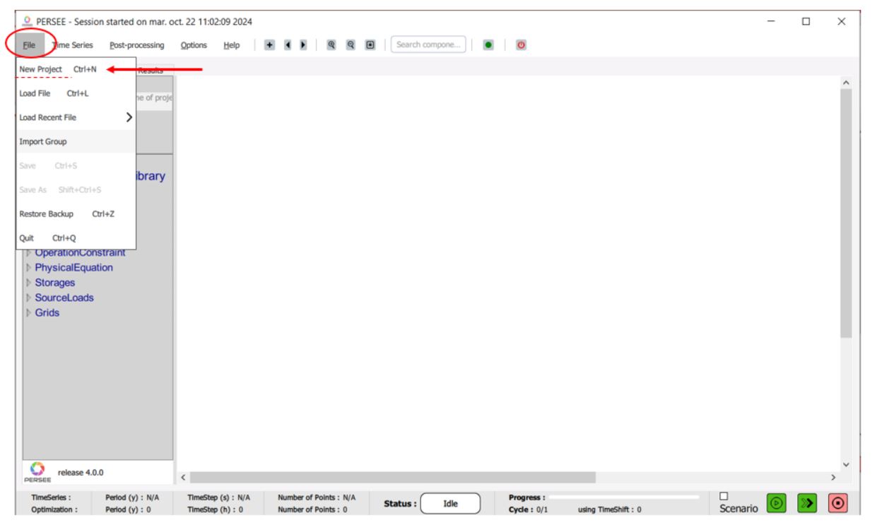
Fig. 27 Creating your first project
Note
At this stage, the Cairn team highly recommends saving your study in a folder with the same name as your project. Since this phase (and future ones) will generate multiple files, it is best practice to keep everything organized in one folder.
Drag and drop components
As the user can see, the Study Data frame now displays your project’s .json file, named after your project. This file has been successfully uploaded into the system.
In the GUI interface, three base components will appear, providing the core structure for building your project. Additionally, the Component Model Library frame, located on the left side of the screen, is now accessible.
As shown in Fig. 28, Cairn organizes the components into four categories. These categories will guide the user in selecting the necessary elements to construct their project.
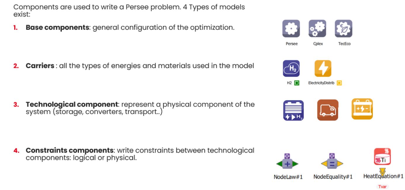
The first category defines the base components, which are essential to define the backbone of the optimization problem (Objective function, Environmental impacts, Optimization algorithm settings and time horizon configuration).
- The second category defines the energy carriers of your problem, and the physical properties associated.
See also
The third category defines the physycal models of your problem. The different modules provided replicate the physical behavior of existant technologies. More information can find in the Submodule Chapter.
The last category defines the constraint components, which allows to set the constraints to your optimization problem.
As it can be seen, Cairn adopts a modular approach, which allows users to model complex energy systems with a high degree of flexibility.
These component blocks can be easily dragged and dropped into the graphical user interface (GUI).
By connecting the components, the user effectively writes the equations governing energy flows, operational limits, and other constraints within the system.
Hint
A highly efficient way of working with Cairn is to first conceptualize the energy system you are studying. Visualize how the different components of the system should be interconnected to achieve the desired energy flow and performance. Once the system is clearly imagined, all you need to do is recreate it in Cairn using the drag-and-drop functionality.
Using Fig. 29 as a reference, you can begin building the energy system in Cairn. Start by identifying the components in the system and dragging the corresponding module from the Component Model Library to the working space on the GUI.
Hint
Better start from the carriers that are going to be used in the system, in order to easily connect later on the components between eachother.
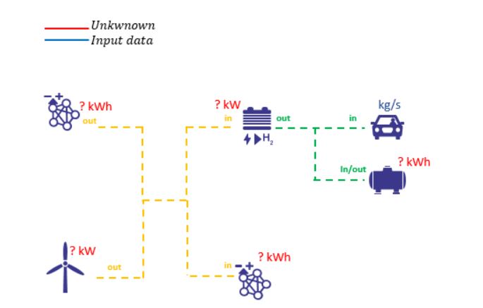
Fig. 29 Sample of the first architecture to be represented
Each module represents a part of the energy system. For example :
If you need a diesel generation unit, drag the module that represents a cogeneration generator.
For energy storage, select the appropriate carrier storage component.
So far, we should have something similar to Fig. 30.
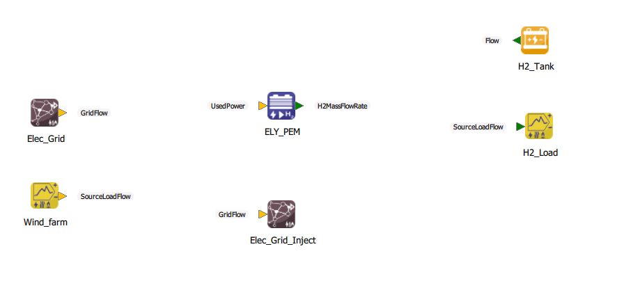
Fig. 30 Drag and drop of components of interest
Now we need to make the connections between the components.
How to link components?
After placing the components, connect them together by defining the carrier that is used by each component. To do so, right click on the arrows and select Set Carrier.
These connections will form the energy balance and set the groundwork for defining the system’s constraints.
As you continue, ensure that the setup of the components mirrors the conceptual system you’ve imagined.
In order to connect the components between eachother and ensure the energy balance, a Node law or a ** NodeEquality** is necessary to perform flow balances ; technological components cannot be connected directly but through buses.
Note
Three types of buses exist:
Node law
NodeEquality
MutliObjective
Note
The energy vector propagates when connecting one port to another: the energy vector of the arrival port automatically aligns with that of the departure port.
There are 3 different types of link. The way to draw them is described below (FigHowToLinks):
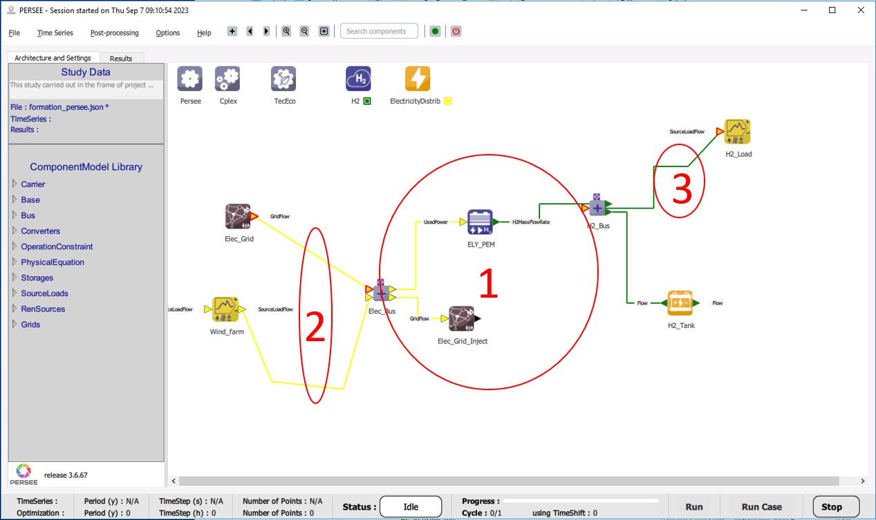
Fig. 31 3 different link types
Horizontal-Vertical segments |
Oblique link |
Hybrid link |
|---|---|---|
Start with click on tail port |
Start with ctrl+click on tail port |
Start with click on tail port |
End with click on head port |
End with click on head port |
End with ctrl+click on head port |
Click to add a point |
Click to add a point |
Click to add a point |
Handle on segment to deplace it |
Handle on segment to split it |
Handle depends on segment type |
Handle on vertex to deplace it |
How to manage big architectures?
The GUI allows to create several pages to manage big architectures.
Each page can hold 150 components.
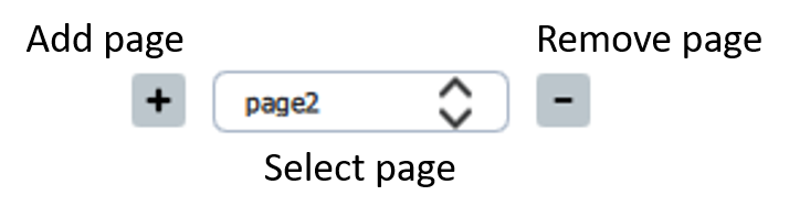
Fig. 32 Pages management, adding a page opens a popup to name the page.
The definition of an energy carrier is shared between all the pages.
Links between the pages can be done through the buses: a bus can be “cloned” by righting clicking on it.
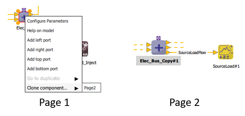
Fig. 33 Cloning a bus to another page in order to be able to add a new port useable in the other page.
Removing a page deletes all the components except the energy vectors used in other pages.
Note
A page can be renamed by right-clicking on an empty space on the page and clicking the Rename page function.
Components (and groups) can be moved between pages in two ways:
Using the context menu: select the components to be moved, right-click on an empty space, choose “Move selection to page”, and then select the target page.
Using keyboard shortcuts: select the components, press Ctrl+X to cut them, navigate to the target page, and press Ctrl+V to paste.
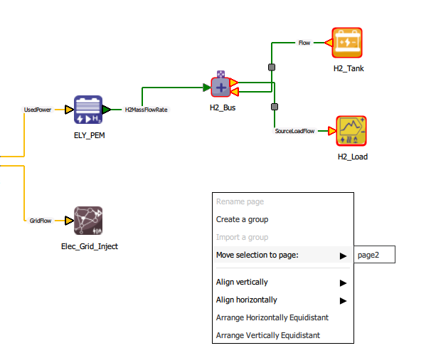
Fig. 34 Move components to another page
How to use groups?
Group of components can be created.
To do so, select all the components that should be in the group. Right click in the page and select “Create a group”.
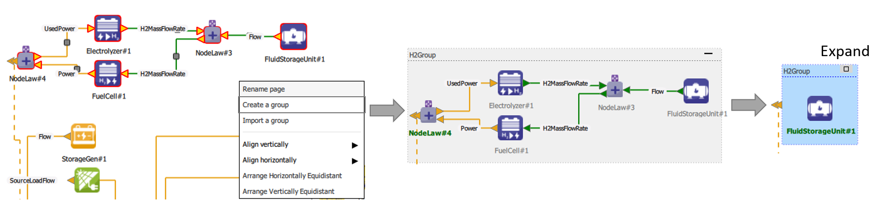
Fig. 35 The steps of a group creation.
Once the group is created, its name can be changed at the top left of it. At the top right, it can be reduced or expanded.
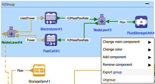
Fig. 36 Different options are available by right clicking inside the group.
The main component that is displayed when the group is reduced can be changed.
The background color can be chosen among a list.
Adding or removing a component inside the group can be done.
Exporting the group can be done. Thus, it saved in .json format and it can be importing in another project in File menu/Import group.
Ungroup the group can also be done here.
Upload the Input time series
Now that the architecture is defined on the GUI, the user can proceed to upload the Input Time Series by using the dedicated drop down menu as showed in Fig. 37.
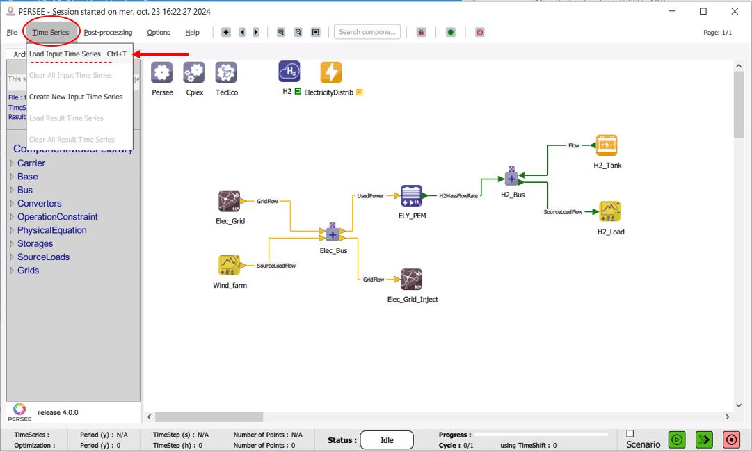
Fig. 37 Loading a time series for input data
After clicking on it, the user will upload the .csv file associated with the proper format. As soon as the Time Series is uploaded, the user can verify if the data has been correcly imported by using the plotter of Cairn.
To do so, click on Results in the left frame Study Data, and then follow the same instructions as for plotting the Results.
See also
Set Model Parameters
Once a model has been drag and dropped on the GUI, and its energy vectors well specified, by double-clicking on it, a list will appear on the board naming the different parameters of the model as showed in the example of Fig. 38.
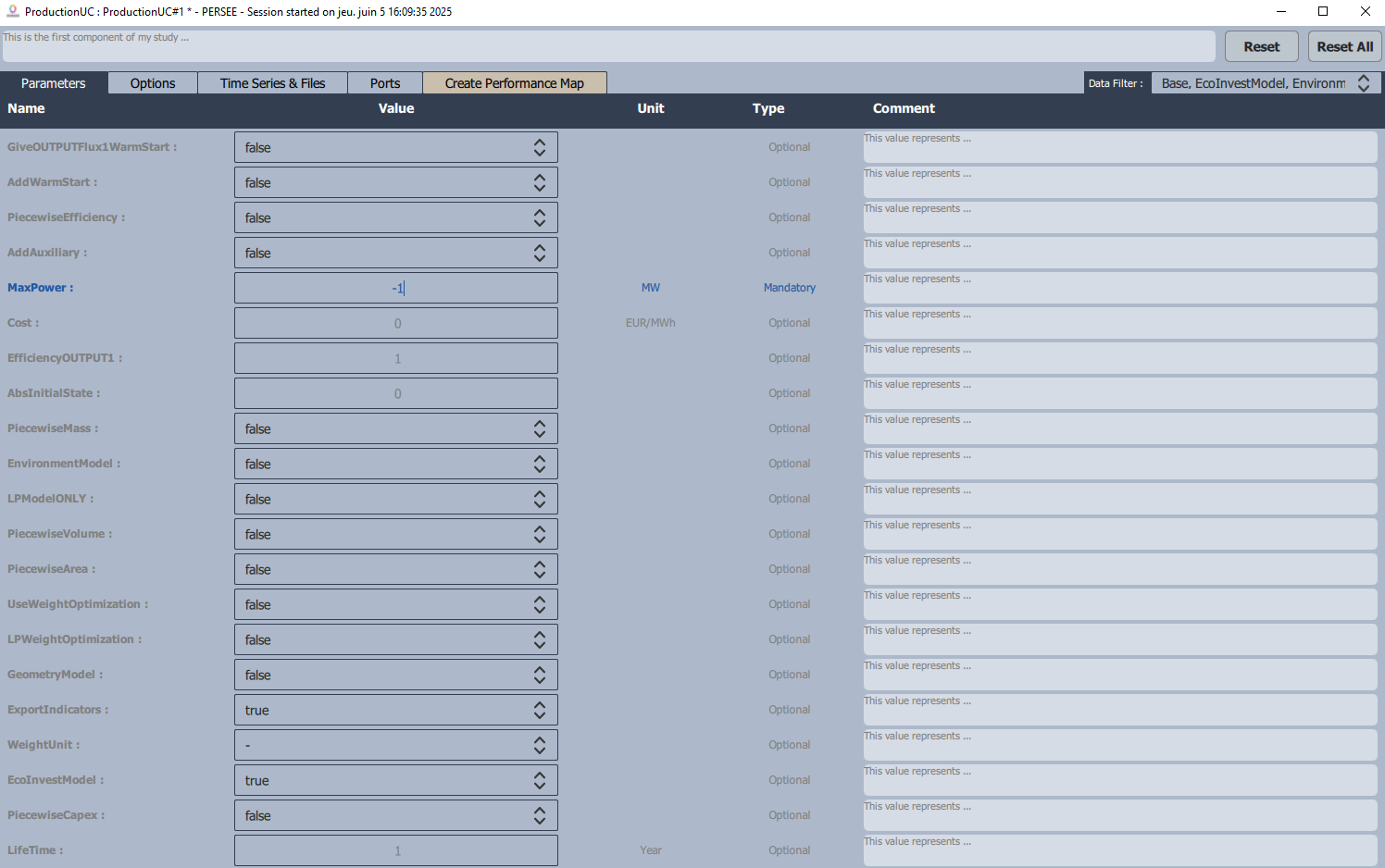
Fig. 38 Parameters window opening when double-clicking right on a component
The parameters that are highlighted in blue are Optimization parameters. The convention used by Cairn to define these variables is the following:
Note
An Optimization variable must be defined with the negative sign. In this why, the user is defining the max value that this variable could have and the min value as 0.
Each component has its own set of parameters depending how it has been modeled. As it can been seen in the upper part of the window, other sections are available. The Time Series & Files section is used to upload into the model the considered time series if needed. Once the time series file have been upload into Cairn (refer to the previous section), the user can find the desired time series in the dropdown menu as shown in Fig. 39.
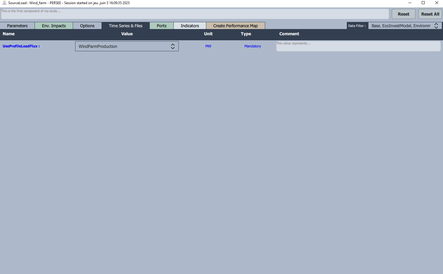
Fig. 39 Uploading the correct timeseries into a component
Note
When finding the timeseries for your component, bear in mind that is very important to be coherent with the unit measure of the timeseries defined in the CSV input file (eg. if the energy vector of your component is electricity, then the component model expect a timeseries input expressed in W).
The Ports section is used to have a clear explanation on how the ports of your model are used, which variables of the model are referred to and if there is a multiplier coefficient that is applied on that variable. In addition, when the EnvironmentalModel parameter is set on True, an additional section to assign environmental parameters is highlighted by a Green Plus Sign on the right.
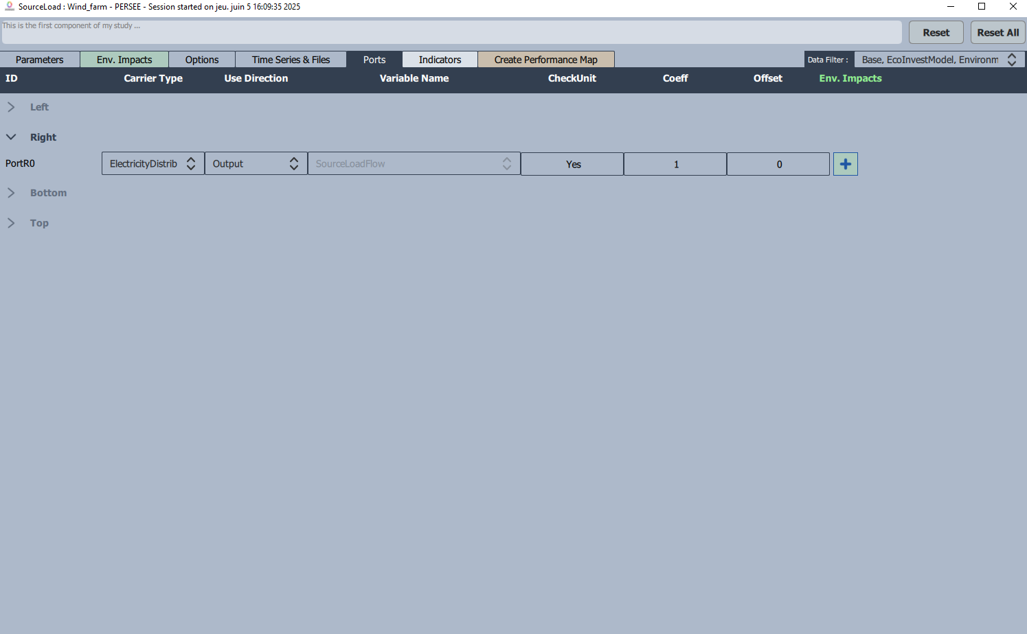
Fig. 40 Ports section
Note
The multiplier coefficient can be used for various operations that are not necesserely implemented in the model itself. For more information, please refere to the section “Advanced usage of a Converter”
Set Base Components Parameters
The Base Components are present from the beginning of the creation of a Cairn project, in the upper left corner.
- TecEco component allows to take into account possible environmental impacts of your case study as well as its lifetime and economic impacts over years.
For more information, please refer to the section Environmental impacts
- |cairn| component defines the timestep of the problem and the optimization time horizon.
For more information, please refer to the section “Rolling Horizon”
- Cplex component is intended to use to have access to the optimization solver and change the parameterization of it.
For more information, please refer to the section “Optimization???”
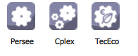
Fig. 41 Base_components
Launch the optimization
Once the time series are correctly upload, the parameters of components are set and objective fixed, the user can launch an optimization process by clicking the green button Run Simulation on the right low corner of the GUI window, as in figure Fig. 42.
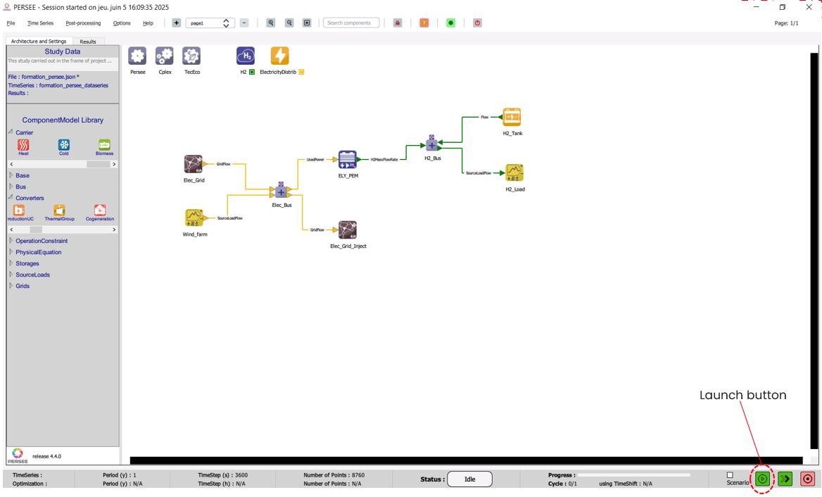
Fig. 42 Launch button
If the user wants to launch only one scenario and name it, it can thick the box on the left of the launch button. A window asking for the name of the particular case under analysis will appear and a folder contaning the results of it will be automatically created by Cairn. The red button on the right of the launch button is a “Stop Simulation” button, which will immediately end the optimization. However, the results of the optimization will be preserved and saved up until the moment the red button has been pushed.